Raymarched Microgeometry on Triangle Meshes
Peter Manohar, Brian Lei, James Fong
Video (YouTube mirror: Mirror)
Abstract
In our project, we present a new rendering technique to efficiently add detail to the surface of triangle meshes. Our method lets us paste any implicit geometry defined via a distance field on top of the surface of a mesh, like a 3D texture. The mesh gives the object its overall shape, and then the “distance field texture” adds the surface detail. Unlike displacement mapping, which can only render heightfield geometry, our method can render any implicit geometry, including non-heightfield geometry. Our method is a hybrid technique, using first a triangle rasterizer and then a raymarcher, and it is highly efficient, allowing us to render very detailed surfaces in real-time. To our knowledge, our rendering technique is new.
Technical approach:
The raymarcher:
Our rendering technique uses raymarching to efficiently render the extra detail on top of surfaces. Raymarching is a rendering technique similar to raytracing that can efficiently render geometry represented by a signed distance field (SDF). A distance field for an implicit surface \(S\) is a function \(f(p)\) that, given a point \(p\) in world-space, returns the distance from \(p\) to the closest point on \(S\). A signed distance field is a distance field, only the returned value is positive if \(p\) lies outside the volume enclosed by \(S\), and negative when \(p\) lies inside the volume enclosed by \(S\).
Raymarching differs from raytracing in how the intersect time of a ray is computed. In raytracing, the intersect time \(t\) is explicitly computed. In raymarching, we instead increase \(t\) in increments until we get within some very small epsilon of the surface, which we count as hitting the surface. By querying the distance field before advancing the ray, we can determine how far we can safely increase \(t\) without passing through the surface and failing to detect the intersection. Many exciting demos illustrating the power of raymarching and distance fields can be found online, for example at http://iquilezles.org/.
Raymarched Microgeometry:
Our goal is to use a raymarcher to efficiently render distance field microgeometry on top of a triangle mesh, like a texture. We will explain how we accomplish this in two steps. We first explain how our method works in the very simple case where the mesh only has one triangle, and then we show how we efficiently generalize our idea to more complicated meshes.
Suppose first that the mesh has only one triangle. We represent the single triangle with a SDF. Then, we render the triangle with added surface detail by doing a two-step raymarch, as follows. In step 1, we raymarch in world coordinates using the triangle SDF until we get within some distance \(\delta\) of the triangle. In step 2, we continue raymarching but in local shell coordinates and with the distance field texture as the SDF, until we get a hit. The shell coordinates of the point \(p_{\text{world}} = (x,y,z)\) are defined as \(p_{\text{shell}} = (u,v,h)\), where \(u\) and \(v\) are the barycentric-interpolated uv texture coordinates of \(p_{\text{world}}\) projected onto the plane containing the triangle, and \(h\) is distance of \(p_{\text{world}}\) to the plane containing the triangle. With this method, we can produce the following images:
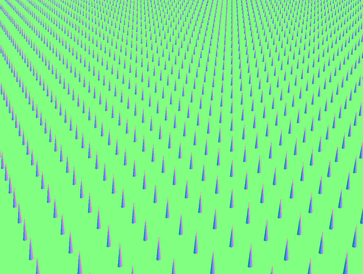 Distance field texture Distance field texture |
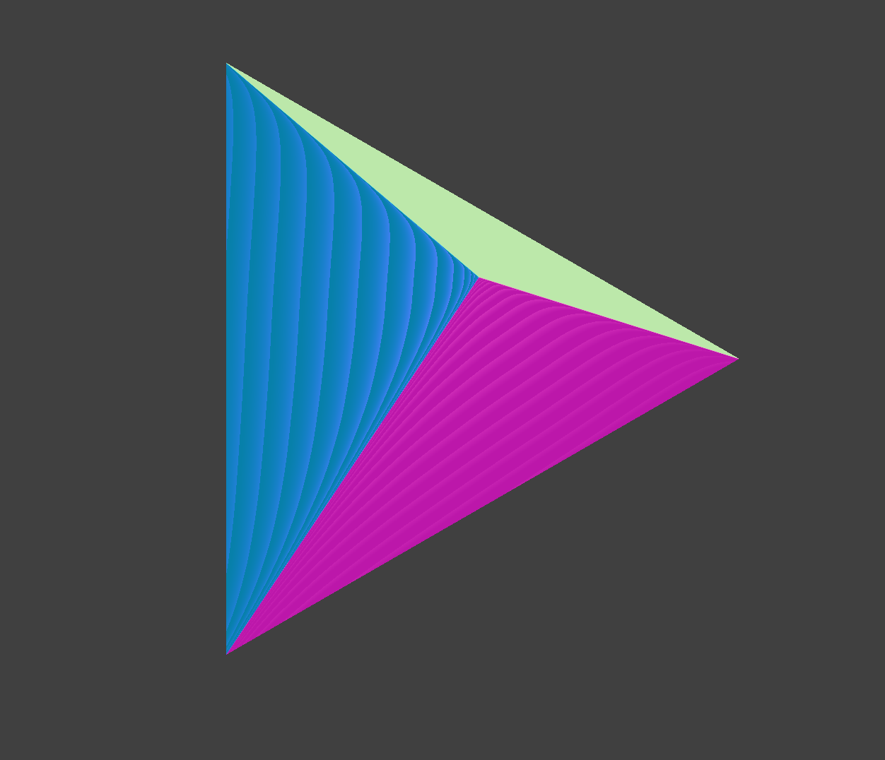 Basic tetrahedron Basic tetrahedron |
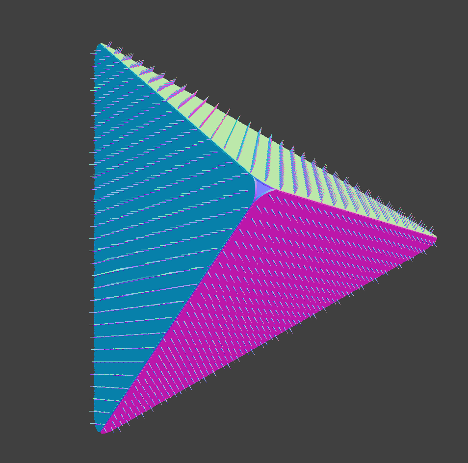 Tetrahedron with distance field texture Tetrahedron with distance field texture |
(Ignore the slight artifact in the image where the corners of the triangle are curved. This artifact doesn’t occur in the final version of our technique, and we didn’t bother fixing it for this intermediate step.)
Unfortunately, this idea becomes prohibitively slow for a large mesh, because we would be converting every triangle into a SDF. Evaluating the SDF would then be very inefficient, similar to how running a ray-intersection test against every triangle in the scene was prohibitively slow in raytracing.
Instead, we generalize the above idea to complicated meshes by using the triangle rasterizer to efficiently execute step 1 (global raymarch) of the raymarcher, where we find the \(\delta\)-radius triangle shell that the ray hits. We do this as follows. We preprocess the mesh by duplicating each vertex and then moving it by distance \(\delta\) along its normal vector. This converts each triangle in the mesh into a small prism, each comprised of three tetrahedrons. Then, we use the rasterizer to “render” the tetrahedrons, and then we do step 2 (local raymarch) in the fragment shader. The z-buffer of the rasterizer provides the efficiency; only the tetrahedrons that will be visible are shaded by the fragment shader, and hence the raymarcher is only used for those fragments.
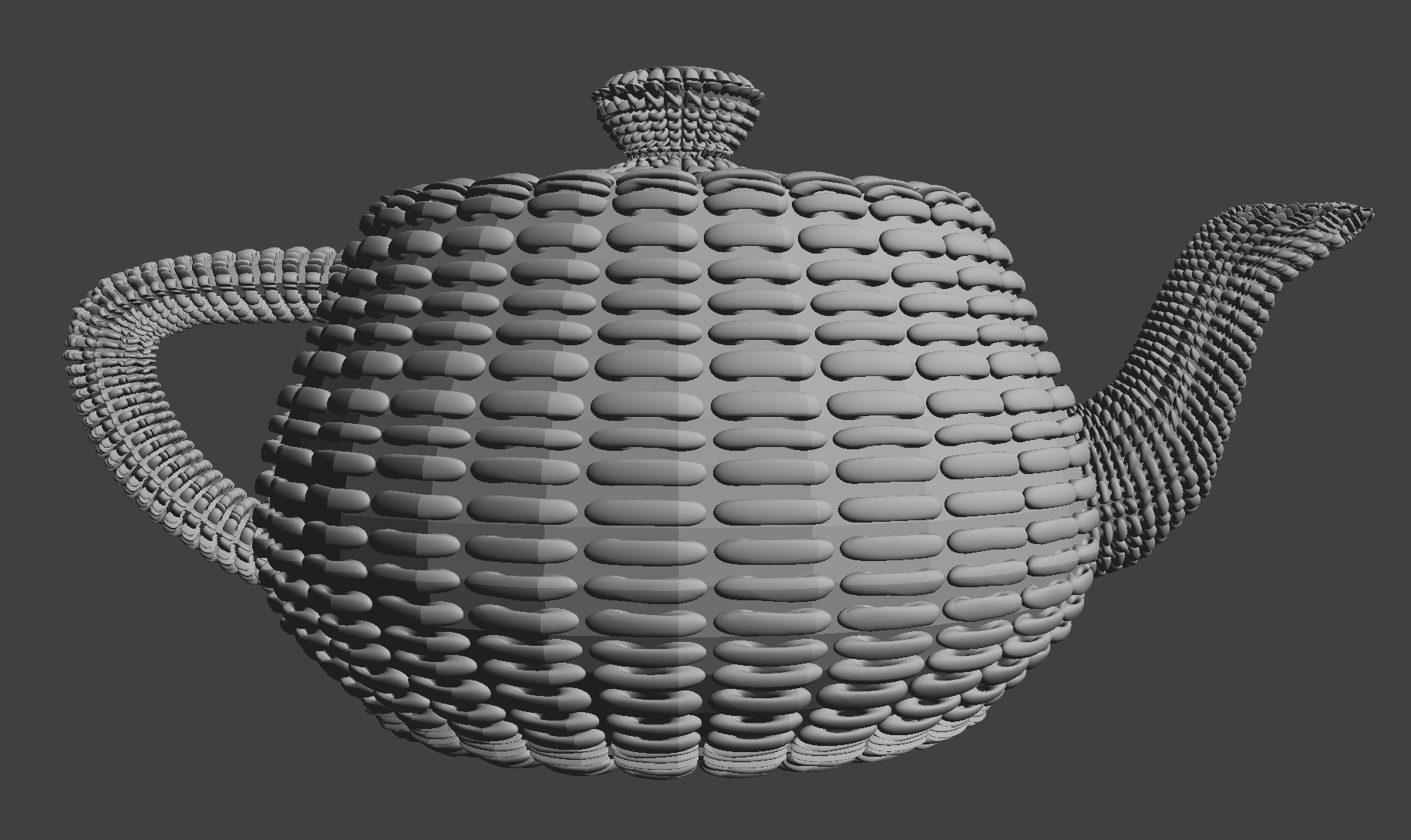
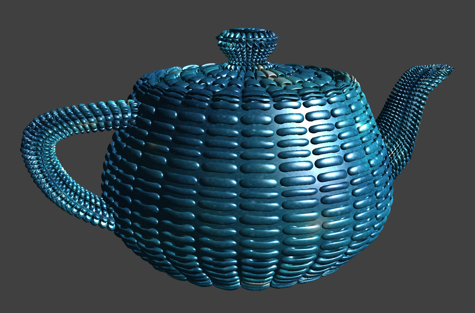
This approach works very well, and can render the teapot below with microgeometry in real time.
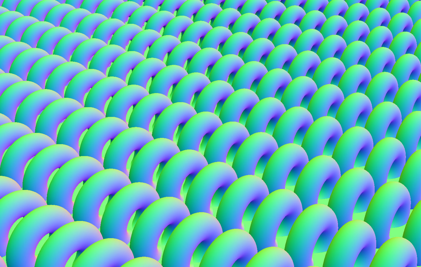 Distance field texture Distance field texture |
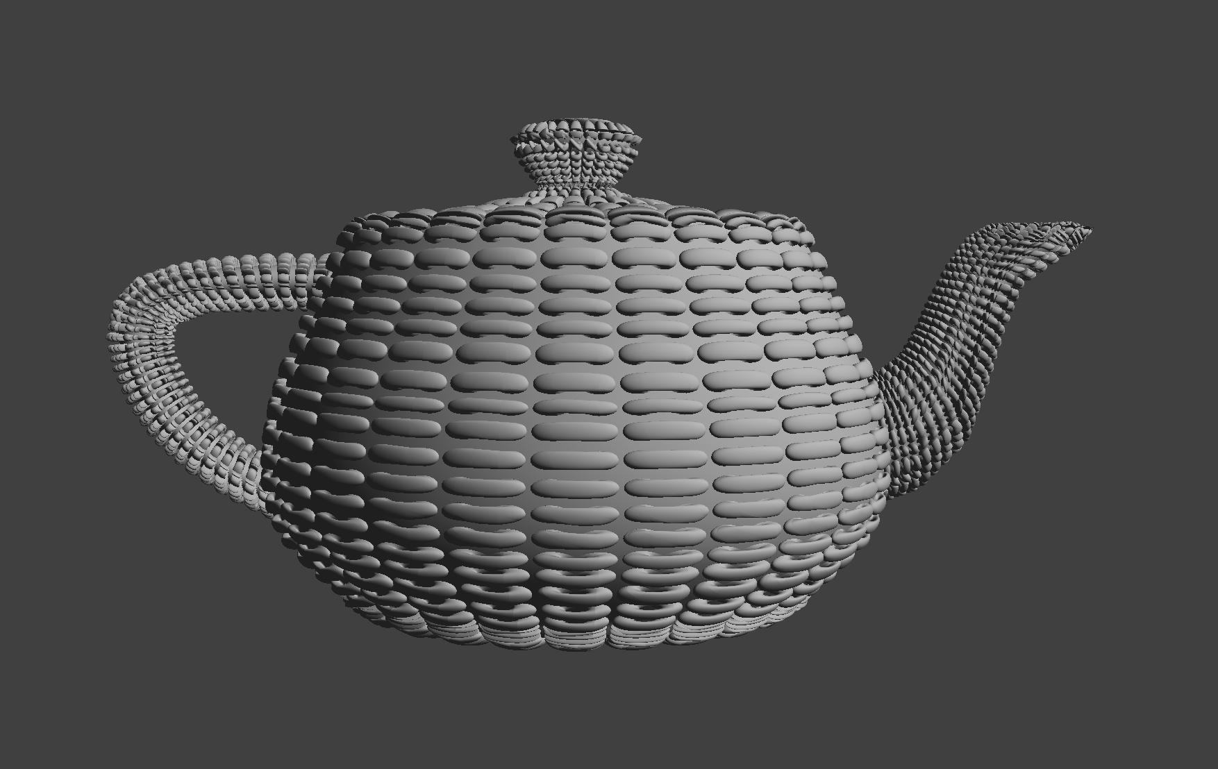 Teapot with distance field texture and diffuse shading Teapot with distance field texture and diffuse shading |
The only problem with the above image is that the microgeometry looks strange near discontinuities in the uv texture coordinates. However, this problem is more of an issue with the way the surface uv coordinates are defined (and this is a general problem with textures), so we ignored it.
Problems Encountered:
Distance field textures extending beyond prisms:
Initially, we encountered an artifact where we would sometimes render distance field texture features beyond the boundaries of the prism. This occurred because the ray casted would miss all the distance field geometry within the prism, but would then hit distance field geometry outside of the prism. We fixed this by checking that our local ray stays within its tetrahedron. If the ray ever exits the tetrahedron, then we kill the ray. The images below show the artifact, why it occurs, and the correct image after the artifact has been fixed.
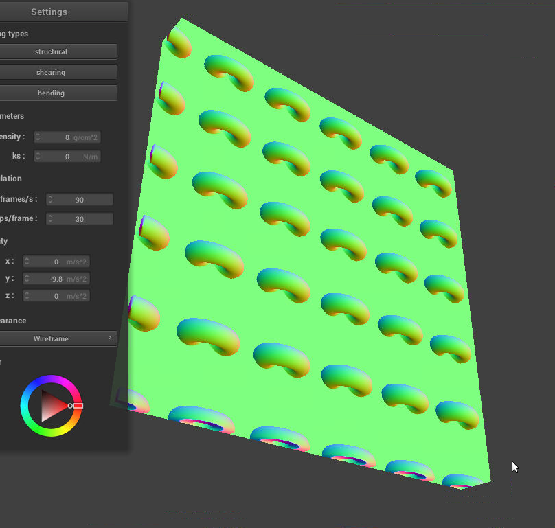 Artifact: plane extends beyond original mesh Artifact: plane extends beyond original mesh |
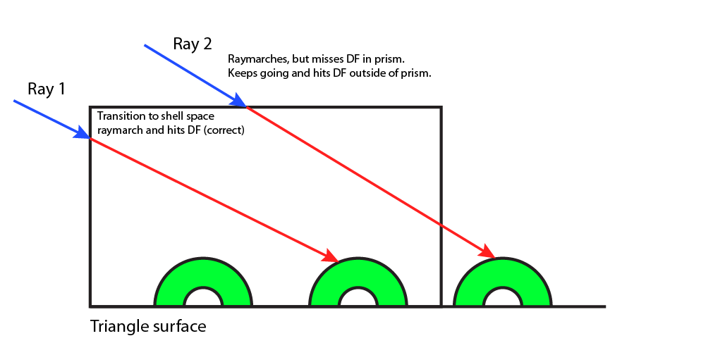 Why the artifact occurs Why the artifact occurs |
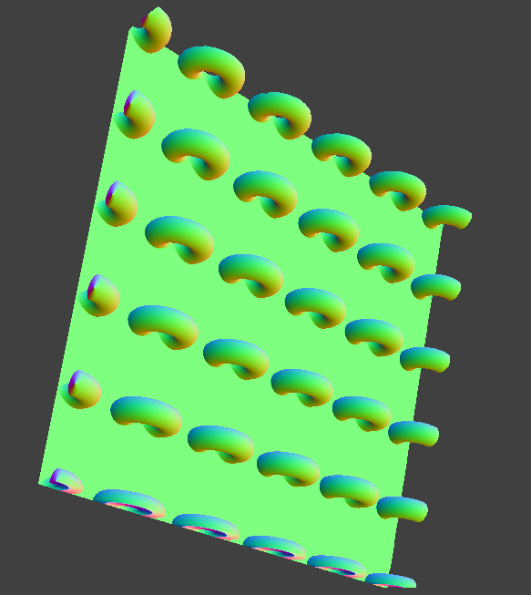 Artifact fixed |
Smoothed normals:
In order to do proper shading, we need the surface normal vectors to be continuous, even across the boundary of the triangles/prisms. If we naively estimate the normal vectors using the distance field, then this property does not hold, and (with a basic diffuse shader) we get the following visual artifact.
 Artifact: normals not smoothed across triangles Artifact: normals not smoothed across triangles |
This artifact is similar to the shading problem we handled in Project 2, which we fixed by using barycentric-interpolated normals rather than triangle-face normals.
Our fix to this problem draws inspiration from the fix in Project 2. Given a point in the prism, we know its triangle-face normal and its barycentric-interpolated normal, and furthermore we can compute a rotation \(R\) that maps the triangle-face normal to the barycentric-interpolated normal. Now, instead of naively returning the distance-field estimated normal (which results in the shading artifact), we instead return \(R\) applied to that normal. With this fix, the shading artifact is gone, and the teapot looks as follows:
| Artifact fixed |
Distance field design and precomputed distance fields:
Designing distance fields is a lot more time-consuming and complicated than it may first appear. A lot of work was spent into designing distance fields that would work well as textures.
Additionally, we implemented 3D precomputed distance fields. Here, we define a distance field that is expensive to compute, and then we sample the distance field at a 3D grid of predetermined points and store the samples in a file. Then, when we wish to render the distance field, we load up the predetermined points and sample them like a 3D texture. This method is a good tool for efficiently rendering complex distance fields, but produces noticeable visual artifacts when the distance field is not sampled with sufficient resolution.
Plant-like fractal microgeometry:
In order to create plant-like microgeometry, we explored (albeit unsuccessfully) Iterated Function Systems (IFSs). Specifically, IFSs are special sets of transformations in mathematics called “contractions” that together define a unique fixed set under the Hutchinson operator called the attractor. This set often exhibits self-similar properties, which is useful for modeling plants, for example. We implemented a chaos game algorithm to generate an approximation of the attractor; a basic outline of the algorithm (with several extensions including 3D shear transforms and noise to increase the variety of models) can be found here.
The idea of the chaos game is that we can start with any initial compact set and apply the transformations randomly. By taking the union of each intermediate result, and taking the number of iterations to infinity, we approach the attractor set.
The main issue here was that we struggled to render the attractor and incorporate it into our pipeline. Our first idea was to use raymarched voxels (grids in 3d space storing point densities). However, this would require us to implement a voxel raymarcher, which we didn’t have time to do. Instead, we decided to precompute a discretized distance field by modeling each point as a small sphere. The main problem with this approach was how to balance efficiency in calculating the distance field with quality. To speed up distance field calculations, we ended up using a BVH structure. Unfortunately, this algorithm didn’t perform very well, as seen in the images below.
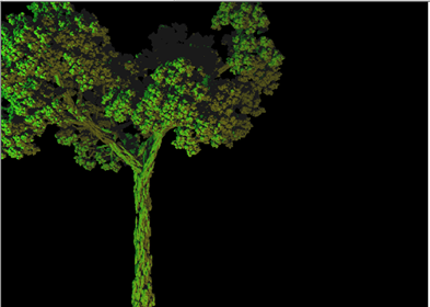 Fractal tree rendered with IFS builder |
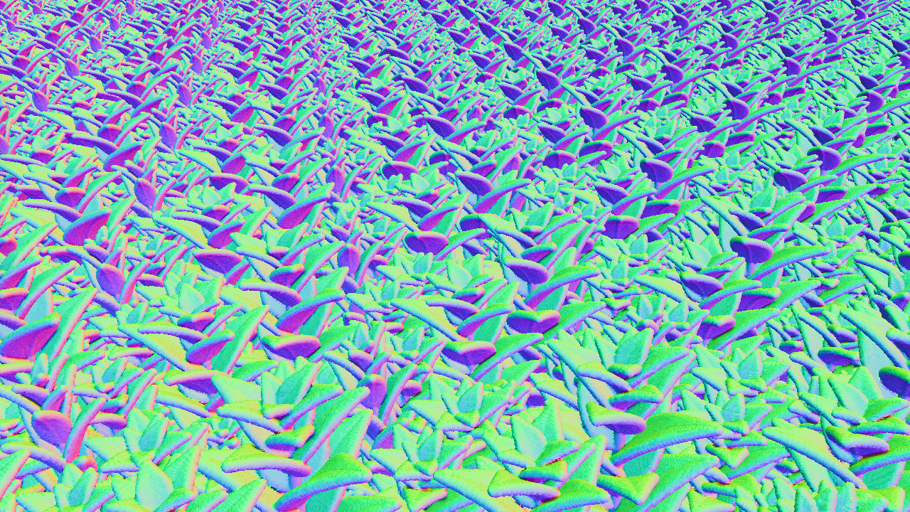
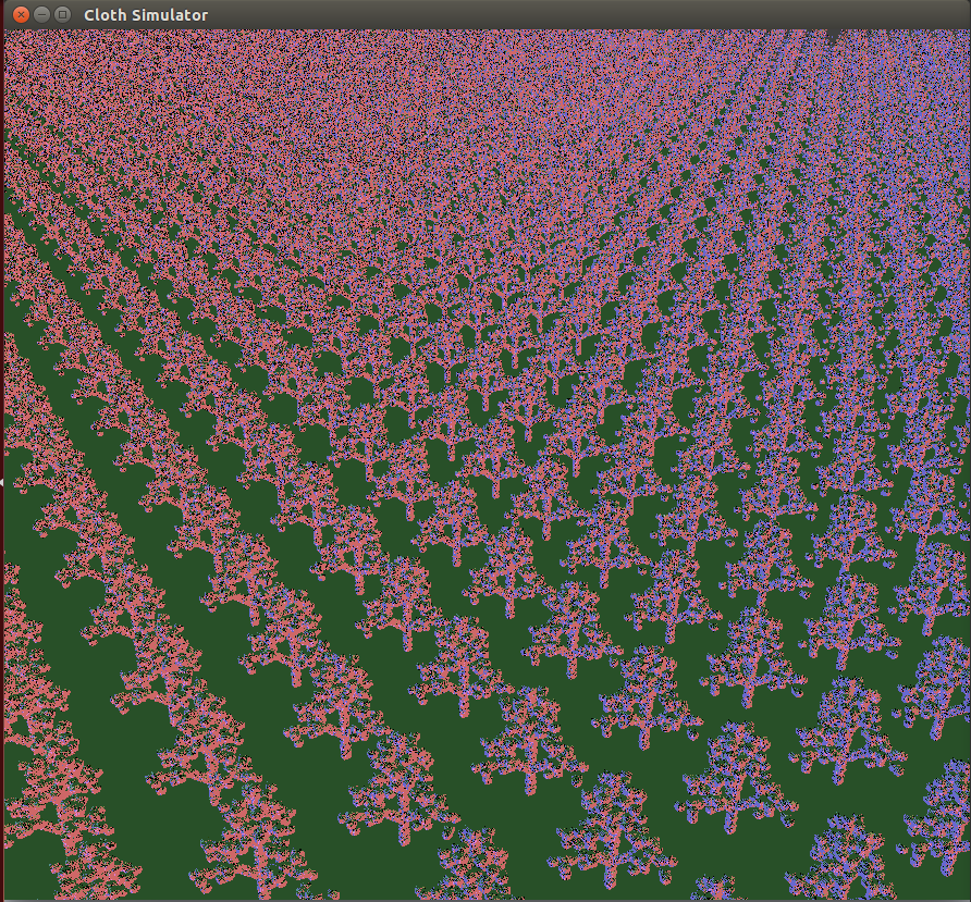 Fractal elm tree distance field texture Fractal elm tree distance field texture |
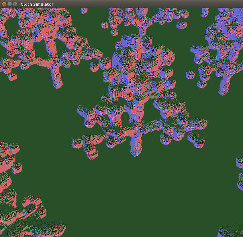 Close up of distance field texture Close up of distance field texture |
Lessons Learned:
The biggest lesson we learned was that, even if an idea sounds good on paper, it doesn’t mean that it will necessarily look good when implemented. For example, our idea of using precomputed and sampled distance fields sounded good on paper, but we ended up needing far too many samples before scenes that we rendered with these distance fields looked visually appealing. Our method of approximating the plant-like fractals using a sampled distance field also sounded great initially, but did not achieve the level of detail that we hoped for, as clearly seen in the images displayed in that section.
Results:
Our rendering method is very powerful and can most likely be used to produce very impressive scenes, if we had the artistic talent to design distance field textures properly. First, we demonstrate our method with a basic teapot scene and a torus distance field texture.
| Distance field texture |
 Teapot with distance field texture and shading Teapot with distance field texture and shading |
Additionally, if we vary the distance field texture with time, we can produce interesting animations. Note that the underlying mesh is static, and only the distance field texture is changing.
Below is the bush scene that was the primary motivation for our project.
 Distance field texture Distance field texture |
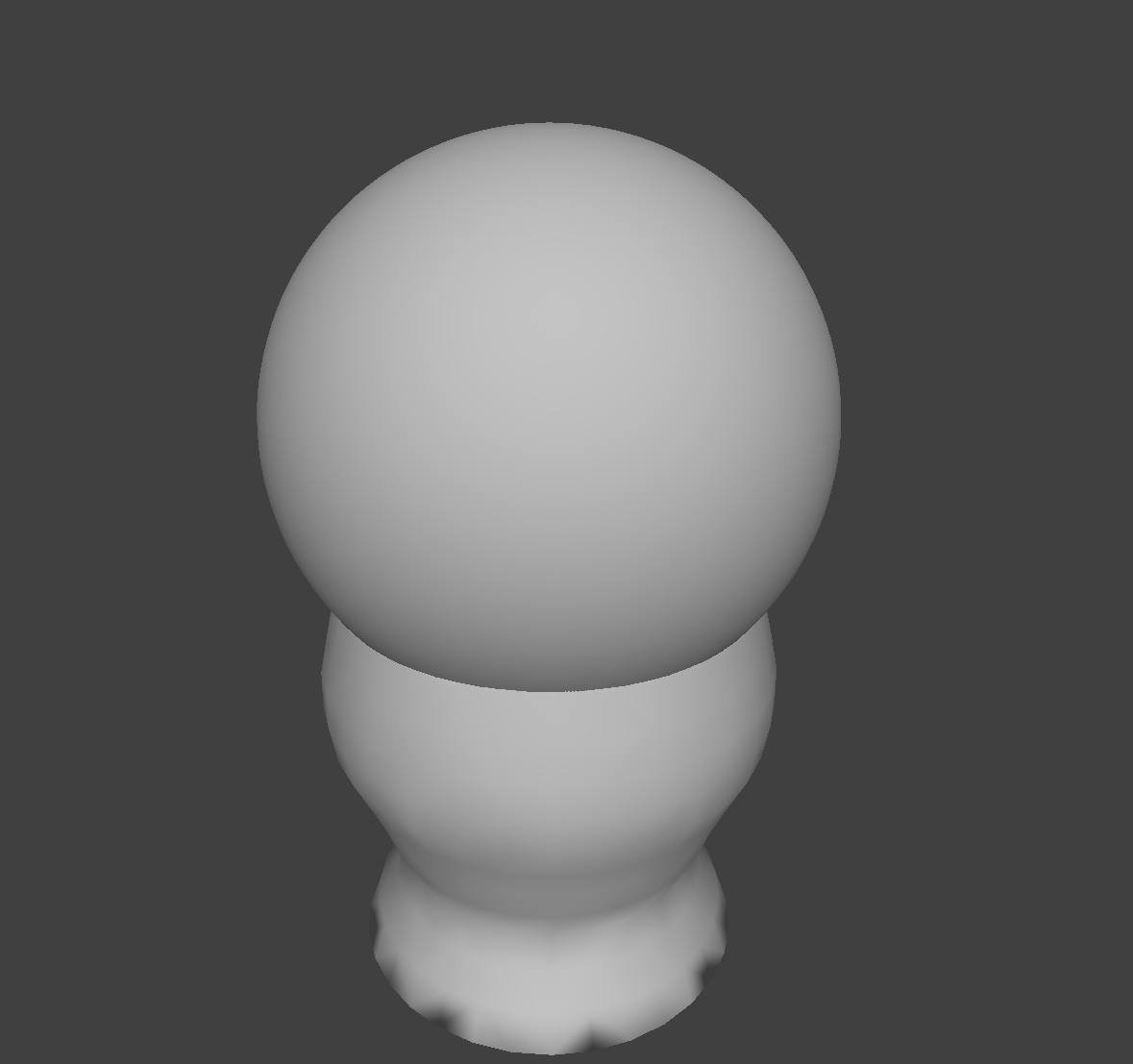 Original Mesh Original Mesh |
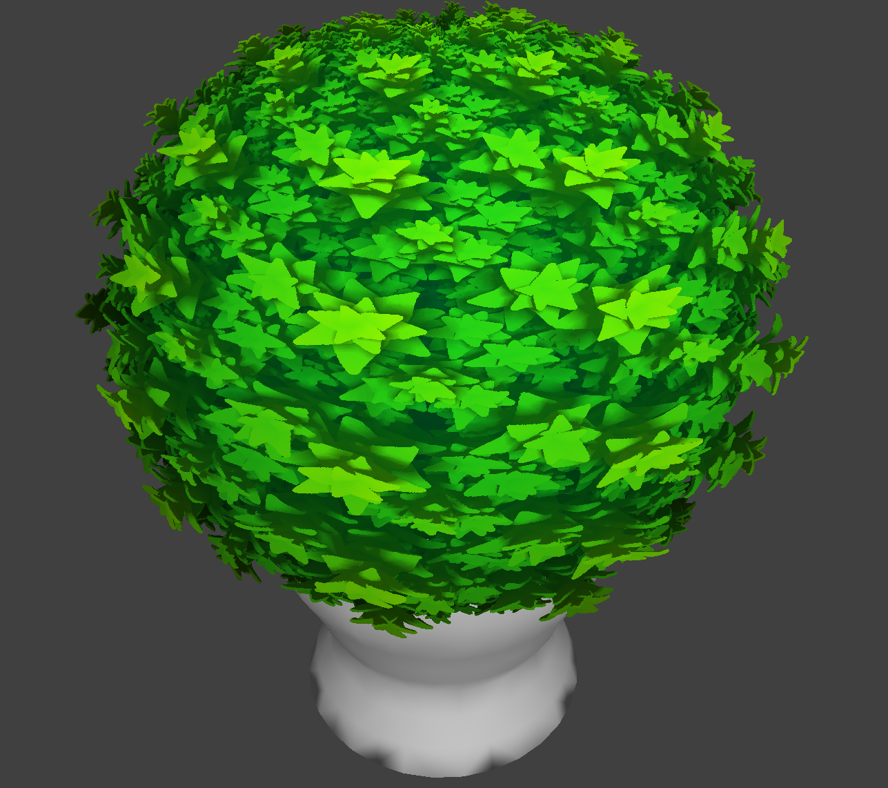 Mesh with distance field texture and shading Mesh with distance field texture and shading |
 Zoom in on detail in bush Zoom in on detail in bush |
This type of added surface detail cannot be achieved by displacement mapping, since the leaves have overhangs and thus are non-heightfield geometry.
References:
Raymarching reference: http://www.iquilezles.org/www/index.htm
IFS and Chaos Game references:
Hart, John C. “Computer Display of Linear Fractal Surfaces.” University of Illinois at Chicago, 1991, www.evl.uic.edu/documents/diss.pdf.
Strnad, D., and N. Guid. “Modeling Trees with Hypertextures.” Computer Graphics Forum, vol. 23, no. 2, 2004, pp. 173–187., http://tume-maailm.pri.ee/ylikool/baka/material/Modeling_Trees_with_Hypertextures.pdf.
We used the clothsim project code as the starter code for our project.
Contributions:
Initially, we had 4 different ideas for how to render the microgeometry:
- Pure distance-field representation,
- Idea 1 with a precomputed distance field,
- Idea 1 using the rasterizer for the global raymarch,
- Use a 4D parameterization of the shell-space SDF
Ideas 1 and 3 were developed jointly by Peter and James. Idea 2 was Peter’s modification of idea 1, and Idea 4 was developed solely by James. Our final implementation uses Idea 3.
James: James worked extensively on the backend C++ code that we used for OpenGL initialization. James implemented ideas 2-4; we used idea 3 as the main technique for rendering scenes with microgeometry, which was implemented entirely by James. James also designed several of the scenes, and helped Brian debug, and he made the final project video. James also implemented the raymarcher over Spring break, before we had even finished writing the project proposal. Honestly, James did so much work on this project that none of us can imagine how he could possibly be taking any other classes.
Peter: Peter implemented idea 1, and helped James find fixes to visual artifacts that James encountered when implementing ideas 2-4. For example, Peter came up with the fixes for the two problems encountered described in the Technical Details section (although James implemented them). He also designed several of the distance field textures and scenes. Peter additionally spent a lot of time working on the presentation of the project. He wrote most of the milestone and final project reports, made the slides and the milestone video, helped James develop the final project video, and he made visually-appealing scenes for use in the final project presentation and video.
Brian: Brian focused on researching ways of efficiently generating and rendering nature models. Brian’s job included calculating tiled distance fields to be used for the microgeometry part the pipeline. Brian successfully implemented the chaos game method for generating IFSs and basic volume partitioning structures, including voxels and BVH, for generating discretized distance fields from IFS point clouds. Ultimately, since we did not implement voxel raymarching, Brian was unable to render his fractals at sufficiently high detail with our distance field raymarcher, so we were unable to use his fractals in our final scenes.